Preview:

A overview of what I will cover in my blog:

1. Data Description
2. Problem Definition
3. Data Preparation
   3.1 Add image label into its file name
   3.2 Create .lmdb data file
   3.3 Compute image mean file .binaryproto using .lmdb file
4. Build network structure
5. Train network
6. Test the network with new images
7. Test Result
8. Tableau report of model performance

0. Get a quick idea about the project achievement before long technical content

I will post a high level description of this project once I get it done

1. Data Description

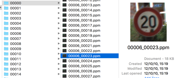
This dataset comes from German Traffic Sign Recognition Benchmark, which contains 39209 images in 43 folders and each folder contain one same kind of traffic sign images taking from different places and at different distance. And the size of the images varies from 30 * 30 pixel to larger than 100 * 100 pixel. Here is how the data fold looks once you download:

2. Problem Definition

Problem type: Image classification

Method: Convolutional Neural Network(CNN)

Software: caffe

Task:

• i. Add image label into its file name
• ii. Using .jpg to create .lmdb data file
• iii. Compute image mean file .binaryproto using .lmdb file
• iv. Build network construction
• v. Train network
• vi. Test the network with new images
• vii. Visualize the test result

3. Data Preparation

3.1 Add image label into its file name

I use two for loops to be able to automatically go through all 43 folders and transfer all .ppm files into .jpg.
Note: transfer image.ppm to image.jpg is not necessary, you can use any format as long as it is supported by openCV to creat .lmdb data file.

for f in range(0,43):
    # save folder name as the format: 00042
    folder = format(f, '05d')
    csv_path = image_root + folder + '/GT-' + folder + '.csv'
    csv = pd.read_csv(csv_path, sep= ';')
    ppm_name = csv['Filename']
    # len(ppm_name) refer to how many .ppm images in each folder
    for i in range(0, len(ppm_name)):
        # select 1/3 as testing image
        if i % 3 == 0:
            im = Image.open(image_root + folder + '/' + csv['Filename'][i])
            im.save('image_path_name' + 'TestJPG/' + format(f, '02d') + '_' +
                    csv['Filename'][i].replace('ppm', 'jpg'))
        else:
            im = Image.open(image_root + folder + '/' + csv['Filename'][i])
            im.save('image_path_name' + 'TrainJPG/' + format(f, '02d') + '_' +
                    csv['Filename'][i].replace('ppm', 'jpg'))

In this step, I separate 1/3 of my dataset into testing images (13070) and the rest as training images (26139) by if the name of the images can be divided by three. And here I add the label of the image(format(f,’02d’)) in front of the image name, which will be helpful to define the label for each image later. Now I have all training images in one folder and so do testing images. Next step is to create lmdb file based on those images.

3.2 Create .lmdb data file

For image preprocessing, I use histogram equalization to the image for adjusting image intensities to enhance contrast and resize the image to 80 * 80.

IMAGE_WIDTH = 80
IMAGE_HEIGHT = 80

def transform_img(img, img_width=IMAGE_WIDTH, img_height=IMAGE_HEIGHT):

    #Histogram Equalization
    img[:, :, 0] = cv2.equalizeHist(img[:, :, 0])
    img[:, :, 1] = cv2.equalizeHist(img[:, :, 1])
    img[:, :, 2] = cv2.equalizeHist(img[:, :, 2])

    #Image Resizing
    img = cv2.resize(img, (img_width, img_height), interpolation = cv2.INTER_CUBIC)

    return img

Here are some comparison before I choose use the size = 80:

Preprocessing	Small image	Big image
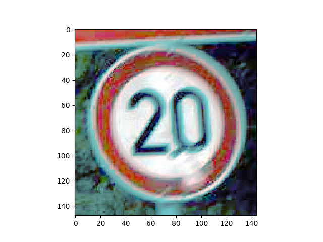
Original images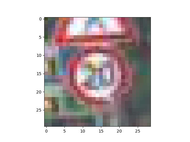
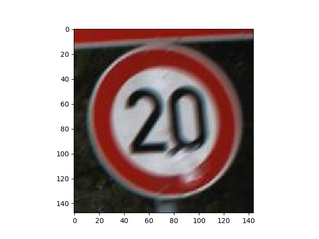Histogram equalization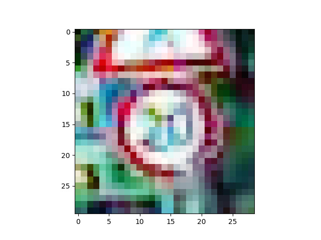
Resize to 50 * 50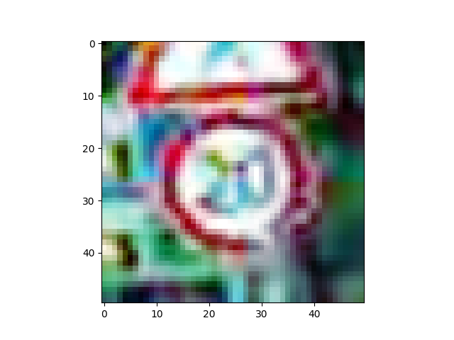
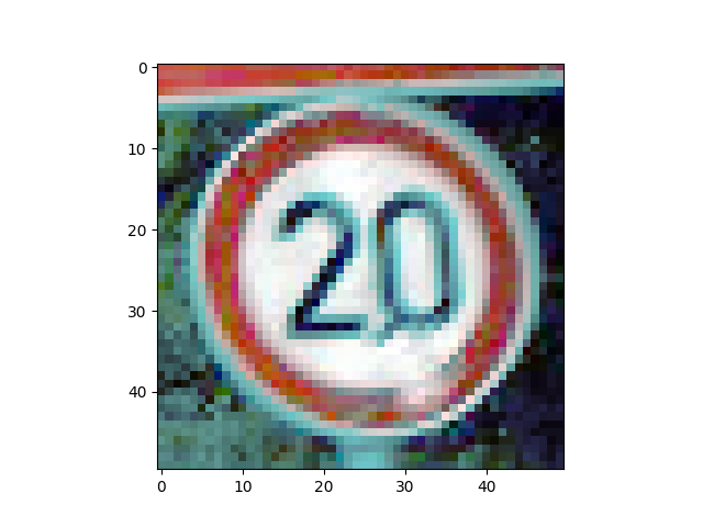Resize to 80 * 80

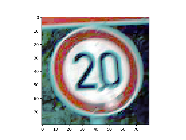Considering my computational power and the clearness of images, I decide to use 80 * 80.

3.3 Compute image mean file .binaryproto using .lmdb file

I use caffe library tool compute_image_mean to compute mean getting mean.binaryproto file.

4. Build network structure

Considering a network layers’ instruction from Stanford CS class CS231n: Convolutional Neural Networks for Visual Recognition:

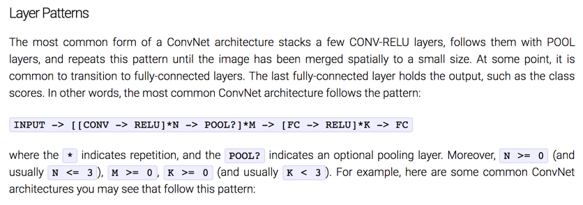
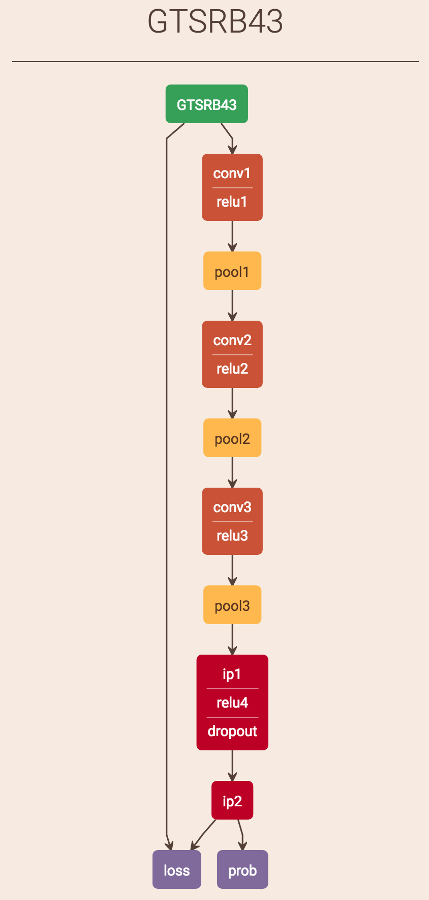
My network structure is the following:

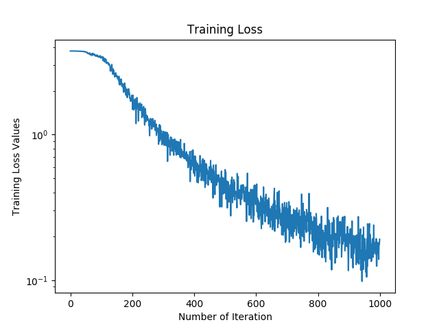
5. Train network

In my training processing, the parameters I use are the following:

test_iter: 50    
test_interval: 1000      
base_lr: 0.001    
momentum: 0.9    
weight_decay: 0.004     
lr_policy: "fixed"  

Training Results

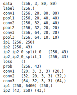
Overview of the network:
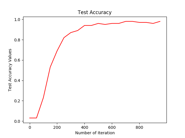
Performance:

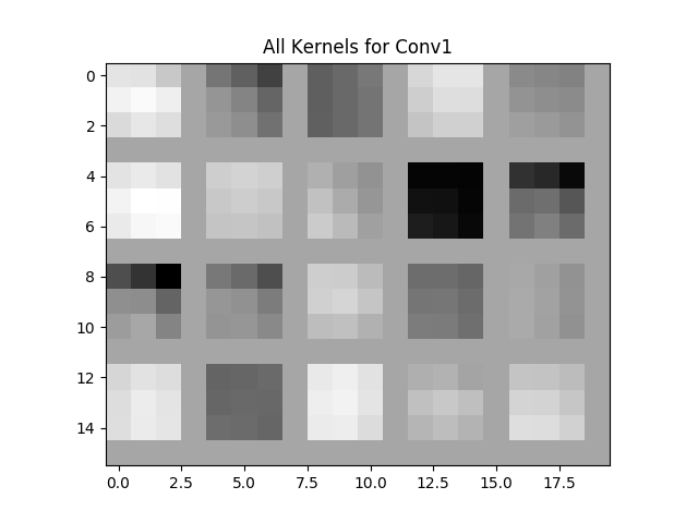
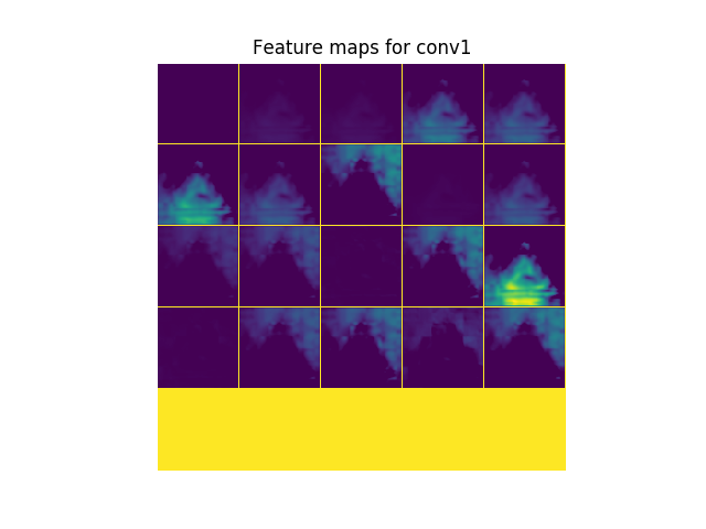
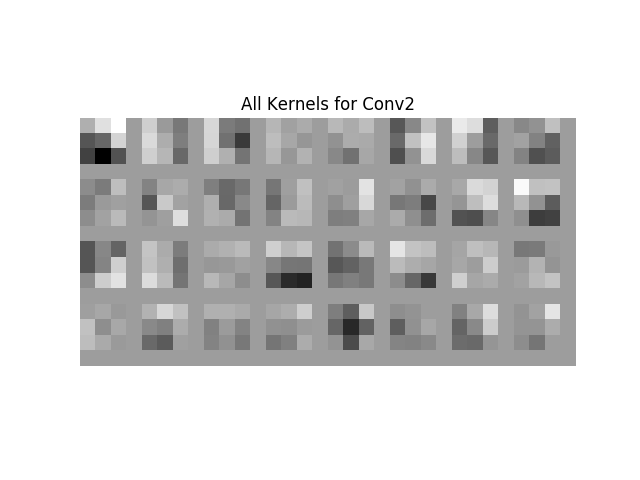
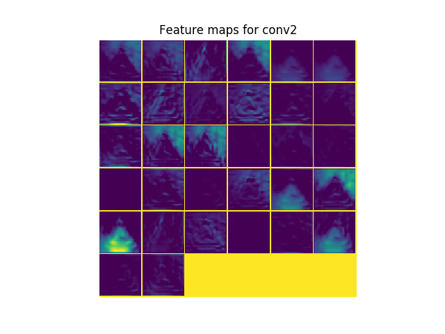
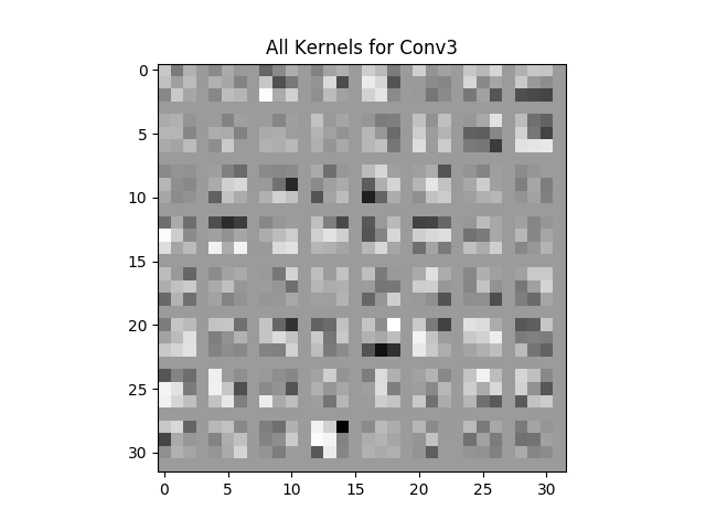
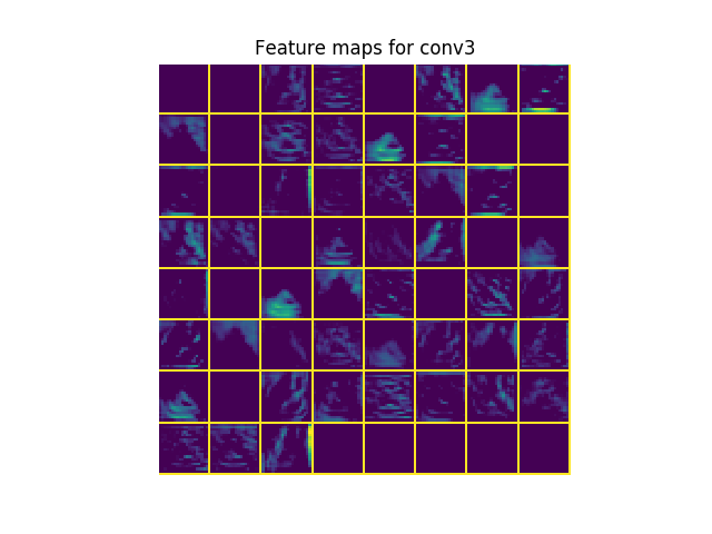
Visualization of kernels and keature maps from all layers:

Kernel	FM

One example output of image recoganiztion with probability of all 43 labels:

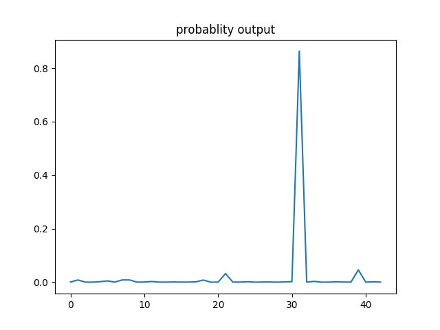
In this example, the image is categotized as label 31 since it has the highest probability.

6. Test the network with new images

To save trained modole can be done by adding just one command:

solver.net.save('Model_43class.caffemodel')

Before we can use the well-trained model to test on any new traffic sign image, there are still some steps need to be finished:

1. Net.prototxt file

(1). Change to input layer instead of data layer that used in training:
Change the following

name: "GTSRB43"
layer {
  name: "GTSRB43"
  type: "Data"
  top: "data"
  top: "label"
  include {
    phase: TRAIN
  }
  transform_param {
    mean_file: "meanTrain.binaryproto"
  }
  data_param {
    source: "train_lmdb"
    batch_size: 64
    backend: LMDB
  }
}

to

name: "GTSRB43Test"
layer {
  name: "TestData"
  type: "Input"
  top: "data"
  input_param { shape: { dim: 1 dim: 3 dim: 80 dim: 80 } }
}

(2). remove outcome layer that depend on label, for example:

layer {
  name: "accuracy"
  type: "Accuracy"
  bottom: "ip2"
  bottom: "label"
  top: "accuracy"
  include {
    phase: TEST
  }
}
layer {
  name: "loss"
  type: "SoftmaxWithLoss"
  bottom: "ip2"
  bottom: "label"
  top: "loss"
}

7. Test Result

The final testset contains 12630 new traffic sign images in random order. Here is my full prediction result:

German Traffic Sign Recognition Benchmark testset prediction

The overall accuracy: 11440 correct predictions out of 12630 (90.58%)

The meaning of columns in my test result:

8. Tableau report of model performance

For better interactive experience, check the dashboard in Tableau

Full code can be found in my github